原创不易,转载请标明出处及原作者。

写在前面的话:本文探讨了在 transformer 模型中使用非线性注意力来预测股票价格的概念。我们讨论了黎曼空间和希尔伯特空间等非线性空间的数学基础,解释了为什么非线性建模可能是有利的,并提供了在代码中实现这种方法的分步指南。
近年来,Transformer 的使用彻底改变了自然语言处理,并越来越多地改变了其他各种领域,例如时间序列分析和股票价格预测。传统的 transformer 架构依赖于线性点积注意力机制,该机制适用于许多任务。但是,这种线性方法可能无法捕获某些数据集(例如股票价格)中关系的全部复杂性,其中非线性依赖关系和复杂模式更为普遍。
一、了解非线性空间:黎曼空间和希尔伯特空间
为了理解为什么非线性注意力机制可能有用,我们需要深入研究几何和泛函分析的一些基本概念。让我们从机器学习中常用的欧几里得空间与黎曼空间和希尔伯特空间等更复杂的空间之间的区别开始。
1. 欧几里得空间
欧几里得空间是我们在初等几何学中学习的熟悉的平面空间。此空间中的距离使用欧几里得距离公式进行测量,点积用于测量向量之间的相似性。在传统的 transformer 中,注意力机制在这个欧几里得空间中运行。
2. 黎曼空间
黎曼空间是允许曲率的欧几里得空间的泛化。在黎曼空间中,测量距离和角度的度量可能因点而异,从而允许空间以复杂的方式弯曲。这种曲率使我们能够对更复杂的关系和依赖关系进行建模,而这些关系和依赖关系在平坦的线性空间中无法充分捕获。
3. 希尔伯特空间
希尔伯特空间是欧几里得空间的无限维泛化,配备了一个完整的内积。它是泛函分析和量子力学中的一个基本概念,为理解具有潜在无限维度的空间提供了一个框架。当我们使用核方法(如 Gaussian 或 Radial Basis Function 内核)时,我们会将数据从有限维欧几里得空间隐式映射到无限维希尔伯特空间。
二、为什么非线性注意力可能是一个好主意
股票价格预测本质上是非线性的。价格受多种因素影响,包括经济指标、新闻事件、投资者情绪和市场微观结构。这些关系通常是复杂的、非线性的和高维的。通过使用非线性注意力机制,我们可以将输入数据映射到更高维的空间,在那里这些复杂的关系可能会变得更加线性且更容易建模。
从本质上讲,使用非线性注意力有助于:
– 捕获数据中复杂的非线性依赖关系。
– 提供更丰富的数据点之间关系表示形式,从而有可能提高预测性能。
– 利用内核函数提供的到更高维度的隐式映射,使我们能够发现线性方法可能遗漏的模式。
三、具有非线性注意力的 Transformer
为了实现具有非线性注意力的 transformer 模型,我们引入了一种基于内核的自定义注意力机制。传统的 transformer 使用点积注意力,这是 inputs 的线性函数。我们的非线性注意力机制使用核函数(例如 Gaussian 或 Radial Basis Function 内核)来计算注意力分数。
非线性注意力机制:
1. 内核注意力层
KernelAttention 类使用查询 (Q) 和键 (K) 矩阵之间的欧几里得距离计算成对距离矩阵。然后使用高斯核转换此距离,该核将数据映射到更高维的空间。结果是反映数据中非线性关系的注意力权重矩阵。
2. 线性注意力层
为了进行比较,我们还使用 PyTorch 的内置 MultiheadAttention 类实现了标准的线性注意力机制。该层对 inputs 执行传统的点积关注。
3. Transformer Decoder 模型
transformer 解码器模型被设计为接受线性和非线性注意力机制,允许我们直接比较它们的有效性。输入序列首先通过线性层将其转换为所需的维数,然后是选定的注意力机制,最后是另一个线性层来输出预测。
四、代码解释
代码实现包括数据加载、预处理、模型定义、训练和评估。以下是关键组件:
1. 数据准备:我们使用 yfinance 库下载 Reliance Industries 的历史股票数据。使用 MinMaxScaler 对数据进行预处理和规范化。
2. 序列创建:使用滑动窗口方法创建输入序列和相应的标签以进行训练。
3. 模型架构:TransformerDecoder 类定义了线性和非线性注意力机制的选项。KernelAttention 类使用 Gaussian 内核实现非线性注意力。
4. 训练和评估:实现了一个 train_model 函数来训练和评估线性和非线性注意力模型。该函数计算训练集和测试集的损失、平均绝对误差 (MAE) 和平均绝对百分比误差 (MAPE)。
5. 可视化:matplotlib 用于绘制损失曲线并比较两个模型的实际价格与预测价格。
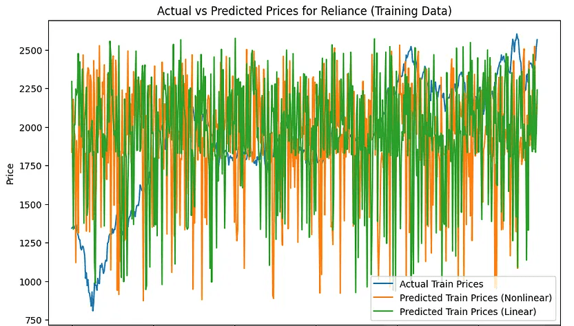
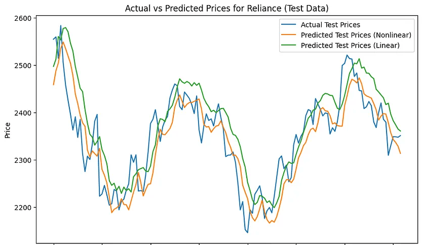
五、结果
非线性注意力:训练集MAE:397.4294,训练集 MAPE:23.40% 非线性注意力:测试集 MAE:39.6702,测试集 MAPE:1.69%
线性注意力:训练集 MAE:397.2669,训练集 MAPE:23.18% 线性注意力:测试集 MAE:48.4979,测试集 MAPE:2.07%
在训练集中
在测试集上
六、结论
通过实现具有非线性注意力的 transformer,与线性注意力机制相比,我们有可能在股票价格数据中捕获更复杂的模式。我们的实验结果提供了两种方法之间的比较,展示了非线性注意力如何在损失、MAE 和 MAPE 方面提供更好的性能。
这种方法展示了从黎曼几何和泛函分析到金融时间序列预测的概念的实际应用。通过利用非线性注意力机制,我们为金融以外的各个领域的复杂关系建模开辟了新的可能性。此处介绍的代码和方法可作为进一步探索和实验的起点。研究人员和从业者可以基于此框架开发更复杂的模型、合并其他功能或将类似技术应用于其他时间序列预测任务。随着我们不断突破机器学习和人工智能的界限,将高级数学概念与实际实现相结合对于开发更强大、更准确的预测模型至关重要。
七、代码
import yfinance as yf
import numpy as np
import pandas as pd
from sklearn.preprocessing import MinMaxScaler
import matplotlib.pyplot as plt
import torch
from torch.utils.data import DataLoader, Dataset
import torch.nn as nn
import torch.nn.functional as F

# Load Reliance historical data
data = yf.download('RELIANCE.NS', start='2020-01-01', end='2023-01-01')

# Preprocess data
data = data[['Close']].dropna()  # Keep only the 'Close' price and drop any missing values

# Normalize the data
scaler = MinMaxScaler(feature_range=(0, 1))
data['Close'] = scaler.fit_transform(data['Close'].values.reshape(-1, 1))

# Create sliding window sequences
def create_sequences(data, window_size):
    sequences = []
    labels = []
    for i in range(len(data) - window_size):
        sequences.append(data[i:i + window_size])
        labels.append(data[i + window_size])
    return np.array(sequences), np.array(labels)

window_size = 30  # Sliding window size of 30 days
X, y = create_sequences(data['Close'].values, window_size)
train_size = int(0.8 * len(X))  # 80% for training
X_train, X_test = X[:train_size], X[train_size:]
y_train, y_test = y[:train_size], y[train_size:]

# Convert data to PyTorch tensors
X_train_tensor = torch.tensor(X_train, dtype=torch.float32).unsqueeze(-1)  # Shape: (batch_size, seq_len, 1)
y_train_tensor = torch.tensor(y_train, dtype=torch.float32).unsqueeze(-1)  # Shape: (batch_size, 1)
X_test_tensor = torch.tensor(X_test, dtype=torch.float32).unsqueeze(-1)    # Shape: (batch_size, seq_len, 1)
y_test_tensor = torch.tensor(y_test, dtype=torch.float32).unsqueeze(-1)    # Shape: (batch_size, 1)

# Create PyTorch Dataset and DataLoader
class TimeSeriesDataset(Dataset):
    def __init__(self, X, y):
        self.X = X
        self.y = y

    def __len__(self):
        return len(self.X)

    def __getitem__(self, idx):
        return self.X[idx], self.y[idx]

train_dataset = TimeSeriesDataset(X_train_tensor, y_train_tensor)
test_dataset = TimeSeriesDataset(X_test_tensor, y_test_tensor)
train_loader = DataLoader(train_dataset, batch_size=32, shuffle=True)
test_loader = DataLoader(test_dataset, batch_size=32, shuffle=False)

# Define a custom kernel attention layer
class KernelAttention(nn.Module):
    def __init__(self, d_model):
        super(KernelAttention, self).__init__()
        self.d_model = d_model
        self.query_layer = nn.Linear(d_model, d_model)
        self.key_layer = nn.Linear(d_model, d_model)
        self.value_layer = nn.Linear(d_model, d_model)

    def forward(self, query, key, value):
        # Ensure correct tensor shapes for debugging
        print(f"Query shape: {query.shape}, Key shape: {key.shape}, Value shape: {value.shape}")

        # Apply linear transformations
        Q = self.query_layer(query)
        K = self.key_layer(key)
        V = self.value_layer(value)

        print(f"Transformed Q shape: {Q.shape}, K shape: {K.shape}, V shape: {V.shape}")

        # Compute pairwise distances and apply Gaussian kernel
        pairwise_distances = torch.cdist(Q, K, p=2)  # Compute pairwise Euclidean distance
        kernel_weights = torch.exp(-pairwise_distances ** 2 / (2 * 0.5 ** 2))  # Gaussian kernel

        # Apply softmax to obtain attention weights
        attention_weights = F.softmax(kernel_weights, dim=-1)
        print(f"Attention weights shape: {attention_weights.shape}")

        # Ensure V has shape (batch_size, seq_len, d_model)
        V = V.view(V.shape[0], -1, self.d_model)  # Reshape V to (batch_size, seq_len, d_model)

        # Compute attention output
        output = torch.bmm(attention_weights, V)  # Shape: (batch_size, seq_len, d_model)
        print(f"Attention output shape: {output.shape}")

        return output

# Define the Transformer Decoder model with Kernel Attention
class TransformerDecoder(nn.Module):
    def __init__(self, window_size, d_model, output_dim):
        super(TransformerDecoder, self).__init__()
        self.kernel_attention = KernelAttention(d_model)
        self.fc1 = nn.Linear(window_size, d_model)
        self.fc2 = nn.Linear(d_model, output_dim)

    def forward(self, x):
        # Reshape input for linear layer
        x = x.view(x.size(0), -1)  # Flatten from (batch_size, seq_len, 1) to (batch_size, seq_len)
        x = self.fc1(x)
        print(f"Input to kernel attention shape: {x.shape}")

        # Reshape x to match expected attention input shape
        x = x.view(x.size(0), -1, self.kernel_attention.d_model)  # Shape: (batch_size, seq_len, d_model)
        x = self.kernel_attention(x, x, x)  # Self-attention
        x = F.relu(x)
        x = torch.mean(x, dim=1)  # Reduce to get fixed output size
        output = self.fc2(x)
        print(f"Model output shape: {output.shape}")

        return output

# Instantiate the model
d_model = 64  # Embedding dimension
output_dim = 1
model = TransformerDecoder(window_size, d_model, output_dim)

# Define loss and optimizer
criterion = nn.MSELoss()
optimizer = torch.optim.Adam(model.parameters(), lr=0.001)

# Training loop
epochs = 20
for epoch in range(epochs):
    model.train()
    total_loss = 0
    for X_batch, y_batch in train_loader:
        optimizer.zero_grad()
        output = model(X_batch)
        loss = criterion(output, y_batch)
        loss.backward()
        optimizer.step()
        total_loss += loss.item()

    print(f"Epoch {epoch+1}/{epochs}, Training Loss: {total_loss / len(train_loader)}")

# Evaluate on test data
model.eval()
test_loss = 0
predictions = []
with torch.no_grad():
    for X_batch, y_batch in test_loader:
        output = model(X_batch)
        loss = criterion(output, y_batch)
        test_loss += loss.item()
        predictions.append(output.numpy())

print(f"Test Loss: {test_loss / len(test_loader)}")

# Convert predictions back to original scale
predictions = np.concatenate(predictions).flatten()
y_test_actual = scaler.inverse_transform(y_test.reshape(-1, 1)).flatten()
predictions_actual = scaler.inverse_transform(predictions.reshape(-1, 1)).flatten()

# Plotting
plt.figure(figsize=(10, 6))
plt.plot(range(len(y_test_actual)), y_test_actual, label='Actual Prices')
plt.plot(range(len(predictions_actual)), predictions_actual, label='Predicted Prices')
plt.xlabel('Time')
plt.ylabel('Price')
plt.title('Actual vs Predicted Prices for Reliance')
plt.legend()
plt.show()

import yfinance as yf
import numpy as np
import pandas as pd
from sklearn.preprocessing import MinMaxScaler
import matplotlib.pyplot as plt
import torch
from torch.utils.data import DataLoader, Dataset
import torch.nn as nn
import torch.nn.functional as F

# Load Reliance historical data
data = yf.download('RELIANCE.NS', start='2020-01-01', end='2023-01-01')

# Preprocess data
data = data[['Close']].dropna()  # Keep only the 'Close' price and drop any missing values

# Normalize the data
scaler = MinMaxScaler(feature_range=(0, 1))
data['Close'] = scaler.fit_transform(data['Close'].values.reshape(-1, 1))

# Create sliding window sequences
def create_sequences(data, window_size):
    sequences = []
    labels = []
    for i in range(len(data) - window_size):
        sequences.append(data[i:i + window_size])
        labels.append(data[i + window_size])
    return np.array(sequences), np.array(labels)

window_size = 30  # Sliding window size of 30 days
X, y = create_sequences(data['Close'].values, window_size)
train_size = int(0.8 * len(X))  # 80% for training
X_train, X_test = X[:train_size], X[train_size:]
y_train, y_test = y[:train_size], y[train_size:]

# Convert data to PyTorch tensors
X_train_tensor = torch.tensor(X_train, dtype=torch.float32).unsqueeze(-1)  # Shape: (batch_size, seq_len, 1)
y_train_tensor = torch.tensor(y_train, dtype=torch.float32).unsqueeze(-1)  # Shape: (batch_size, 1)
X_test_tensor = torch.tensor(X_test, dtype=torch.float32).unsqueeze(-1)    # Shape: (batch_size, seq_len, 1)
y_test_tensor = torch.tensor(y_test, dtype=torch.float32).unsqueeze(-1)    # Shape: (batch_size, 1)

# Create PyTorch Dataset and DataLoader
class TimeSeriesDataset(Dataset):
    def __init__(self, X, y):
        self.X = X
        self.y = y

    def __len__(self):
        return len(self.X)

    def __getitem__(self, idx):
        return self.X[idx], self.y[idx]

train_dataset = TimeSeriesDataset(X_train_tensor, y_train_tensor)
test_dataset = TimeSeriesDataset(X_test_tensor, y_test_tensor)
train_loader = DataLoader(train_dataset, batch_size=32, shuffle=True)
test_loader = DataLoader(test_dataset, batch_size=32, shuffle=False)

# Define a custom kernel attention layer
class KernelAttention(nn.Module):
    def __init__(self, d_model):
        super(KernelAttention, self).__init__()
        self.d_model = d_model
        self.query_layer = nn.Linear(d_model, d_model)
        self.key_layer = nn.Linear(d_model, d_model)
        self.value_layer = nn.Linear(d_model, d_model)

    def forward(self, query, key, value):
        # Apply linear transformations
        Q = self.query_layer(query)
        K = self.key_layer(key)
        V = self.value_layer(value)

        # Compute pairwise distances and apply Gaussian kernel
        pairwise_distances = torch.cdist(Q, K, p=2)  # Compute pairwise Euclidean distance
        kernel_weights = torch.exp(-pairwise_distances ** 2 / (2 * 0.5 ** 2))  # Gaussian kernel

        # Apply softmax to obtain attention weights
        attention_weights = F.softmax(kernel_weights, dim=-1)

        # Ensure V has shape (batch_size, seq_len, d_model)
        V = V.view(V.shape[0], -1, self.d_model)  # Reshape V to (batch_size, seq_len, d_model)

        # Compute attention output
        output = torch.bmm(attention_weights, V)  # Shape: (batch_size, seq_len, d_model)

        return output

# Define the Linear Attention layer for comparison
class LinearAttention(nn.Module):
    def __init__(self, d_model):
        super(LinearAttention, self).__init__()
        self.d_model = d_model
        self.attention = nn.MultiheadAttention(embed_dim=d_model, num_heads=1)

    def forward(self, query, key, value):
        query = query.permute(1, 0, 2)  # Rearrange for attention layer (seq_len, batch_size, d_model)
        key = key.permute(1, 0, 2)
        value = value.permute(1, 0, 2)

        # Perform standard multi-head self-attention
        output, _ = self.attention(query, key, value)
        output = output.permute(1, 0, 2)  # Rearrange back to (batch_size, seq_len, d_model)
        return output

# Define the Transformer Decoder model with both attentions
class TransformerDecoder(nn.Module):
    def __init__(self, window_size, d_model, output_dim, attention_type='nonlinear'):
        super(TransformerDecoder, self).__init__()
        if attention_type == 'nonlinear':
            self.attention_layer = KernelAttention(d_model)
        elif attention_type == 'linear':
            self.attention_layer = LinearAttention(d_model)
        else:
            raise ValueError("Unsupported attention type. Choose either 'linear' or 'nonlinear'.")

        self.fc1 = nn.Linear(window_size, d_model)
        self.fc2 = nn.Linear(d_model, output_dim)

    def forward(self, x):
        # Reshape input for linear layer
        x = x.view(x.size(0), -1)  # Flatten from (batch_size, seq_len, 1) to (batch_size, seq_len)
        x = self.fc1(x)

        # Reshape x to match expected attention input shape
        x = x.view(x.size(0), -1, self.attention_layer.d_model)  # Shape: (batch_size, seq_len, d_model)
        x = self.attention_layer(x, x, x)  # Attention mechanism
        x = F.relu(x)
        x = torch.mean(x, dim=1)  # Reduce to get fixed output size
        output = self.fc2(x)

        return output

# Train and evaluate both models
def train_model(attention_type):
    # Instantiate the model
    d_model = 64  # Embedding dimension
    output_dim = 1
    model = TransformerDecoder(window_size, d_model, output_dim, attention_type=attention_type)

    # Define loss and optimizer
    criterion = nn.MSELoss()
    optimizer = torch.optim.Adam(model.parameters(), lr=0.001)

    # Training loop
    epochs = 20
    train_losses = []
    test_losses = []

    for epoch in range(epochs):
        model.train()
        total_loss = 0
        for X_batch, y_batch in train_loader:
            optimizer.zero_grad()
            output = model(X_batch)
            loss = criterion(output, y_batch)
            loss.backward()
            optimizer.step()
            total_loss += loss.item()
        train_losses.append(total_loss / len(train_loader))
        print(f"Epoch {epoch+1}/{epochs} ({attention_type}), Training Loss: {train_losses[-1]}")

        # Evaluate on test data
        model.eval()
        test_loss = 0
        with torch.no_grad():
            for X_batch, y_batch in test_loader:
                output = model(X_batch)
                loss = criterion(output, y_batch)
                test_loss += loss.item()
        test_losses.append(test_loss / len(test_loader))
        print(f"Epoch {epoch+1}/{epochs} ({attention_type}), Test Loss: {test_losses[-1]}")

    # Get predictions for train and test data
    model.eval()
    train_predictions = []
    test_predictions = []

    with torch.no_grad():
        for X_batch, _ in train_loader:
            train_output = model(X_batch)
            train_predictions.append(train_output.numpy())

        for X_batch, _ in test_loader:
            test_output = model(X_batch)
            test_predictions.append(test_output.numpy())

    train_predictions = np.concatenate(train_predictions).flatten()
    test_predictions = np.concatenate(test_predictions).flatten()

    # Convert predictions back to original scale
    y_train_actual = scaler.inverse_transform(y_train.reshape(-1, 1)).flatten()
    y_test_actual = scaler.inverse_transform(y_test.reshape(-1, 1)).flatten()
    train_predictions_actual = scaler.inverse_transform(train_predictions.reshape(-1, 1)).flatten()
    test_predictions_actual = scaler.inverse_transform(test_predictions.reshape(-1, 1)).flatten()

    # Calculate MAE and MAPE
    mae_train = np.mean(np.abs(y_train_actual - train_predictions_actual))
    mae_test = np.mean(np.abs(y_test_actual - test_predictions_actual))
    mape_train = np.mean(np.abs((y_train_actual - train_predictions_actual) / y_train_actual)) * 100
    mape_test = np.mean(np.abs((y_test_actual - test_predictions_actual) / y_test_actual)) * 100

    print(f"Train MAE ({attention_type}): {mae_train:.4f}, Train MAPE ({attention_type}): {mape_train:.2f}%")
    print(f"Test MAE ({attention_type}): {mae_test:.4f}, Test MAPE ({attention_type}): {mape_test:.2f}%")

    return train_losses, test_losses, y_train_actual, train_predictions_actual, y_test_actual, test_predictions_actual, mae_train, mape_train, mae_test, mape_test

# Train and evaluate nonlinear attention
train_losses_nonlinear, test_losses_nonlinear, y_train_actual, train_predictions_actual_nonlinear, y_test_actual, test_predictions_actual_nonlinear, mae_train_nonlinear, mape_train_nonlinear, mae_test_nonlinear, mape_test_nonlinear = train_model('nonlinear')

# Train and evaluate linear attention
train_losses_linear, test_losses_linear, _, train_predictions_actual_linear, _, test_predictions_actual_linear, mae_train_linear, mape_train_linear, mae_test_linear, mape_test_linear = train_model('linear')

# Plot the loss curves for both models
plt.figure(figsize=(10, 6))
plt.plot(train_losses_nonlinear, label='Training Loss (Nonlinear Attention)')
plt.plot(test_losses_nonlinear, label='Test Loss (Nonlinear Attention)')
plt.plot(train_losses_linear, label='Training Loss (Linear Attention)')
plt.plot(test_losses_linear, label='Test Loss (Linear Attention)')
plt.xlabel('Epochs')
plt.ylabel('Loss')
plt.title('Training and Test Loss Curves for Nonlinear and Linear Attention')
plt.legend()
plt.show()

# Plot predictions for both models
plt.figure(figsize=(10, 6))
plt.plot(range(len(y_train_actual)), y_train_actual, label='Actual Train Prices')
plt.plot(range(len(train_predictions_actual_nonlinear)), train_predictions_actual_nonlinear, label='Predicted Train Prices (Nonlinear)')
plt.plot(range(len(train_predictions_actual_linear)), train_predictions_actual_linear, label='Predicted Train Prices (Linear)')
plt.xlabel('Time')
plt.ylabel('Price')
plt.title('Actual vs Predicted Prices for Reliance (Training Data)')
plt.legend()
plt.show()

plt.figure(figsize=(10, 6))
plt.plot(range(len(y_test_actual)), y_test_actual, label='Actual Test Prices')
plt.plot(range(len(test_predictions_actual_nonlinear)), test_predictions_actual_nonlinear, label='Predicted Test Prices (Nonlinear)')
plt.plot(range(len(test_predictions_actual_linear)), test_predictions_actual_linear, label='Predicted Test Prices (Linear)')
plt.xlabel('Time')
plt.ylabel('Price')
plt.title('Actual vs Predicted Prices for Reliance (Test Data)')
plt.legend()
plt.show()

# Print comparison of MAE and MAPE
print(f"Nonlinear Attention: Train MAE: {mae_train_nonlinear:.4f}, Train MAPE: {mape_train_nonlinear:.2f}%")
print(f"Nonlinear Attention: Test MAE: {mae_test_nonlinear:.4f}, Test MAPE: {mape_test_nonlinear:.2f}%")
print(f"Linear Attention: Train MAE: {mae_train_linear:.4f}, Train MAPE: {mape_train_linear:.2f}%")
print(f"Linear Attention: Test MAE: {mae_test_linear:.4f}, Test MAPE: {mape_test_linear:.2f}%")
本文内容仅仅是技术探讨和学习,并不构成任何投资建议。
转发请注明原作者和出处。
Be First to Comment