作者:老余捞鱼
原创不易,转载请标明出处及原作者。

写在前面的话:本文介绍了如何使用 Python 和专业数据源(如 Alpha Vantage)来获取高质量数据,以及如何构建和分析量化交易策略,特别是开盘区间突破(ORB)策略,并通过实际代码示例展示了如何计算价格缺口、成交量、移动平均线等关键指标,以帮助入门数据交易者做出更简单的交易决策。
如果您着手准备开始使用 Python 编写股票交易算法,那么您将面临的最紧迫问题是:我需要什么样的数据,我在哪里可以找到这些数据。我花了很多时间来研究这个问题,很乐意为您提供帮助。
在本文中,我们将构建一个超级全面的数据框架,其中包含创建制胜算法所需的一切。但更重要的是,我在这里分享的代码设计得非常容易适应不同的时间框架,希望你在需要抓取自己的数据时可以重复使用。
市面上有很多股票数据 API,但对于定量分析,我推荐 https://www.alphavantage.co/,因为它带来了很多已经计算好的指标,而且盘中粒度可达 1 分钟,这是定量分析人员的必备工具。
具体内容可以看我这篇文章:《手把手教你ai顾投:发现一个高质量的金融数据源》
一、获取数据
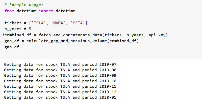
下面的代码将自动抓取您选择的股票数据,并将它们连接到一个数据框中:
!pip install alpha_vantage
from datetime import datetime
from datetime import timedelta

from alpha_vantage.timeseries import TimeSeries
import requests
import pandas as pd
import numpy as np
import datetime
from re import M
import requests
api_key = 'MY_ALPHA_VANTAGE_KEY'

def get_last_n_years_months(n):
    current_date = datetime.now()
    start_date = current_date - timedelta(days=n*365)  # Approximate start date n years ago
    months = []

    while start_date <= current_date:
        month = start_date.strftime('%Y-%m')
        months.append(month)
        start_date += timedelta(days=32)  # Move to the next month
        start_date = start_date.replace(day=1)  # Set to the first day of the next month

    return months

def fetch_stock_data(ticker, n_years, api_key):
    period = get_last_n_years_months(n_years)
    final_df = pd.DataFrame()

    for i in period:
        print(f'Getting data for stock {ticker} and period {i}')
        url = f'https://www.alphavantage.co/query?function=TIME_SERIES_INTRADAY&symbol={ticker}&interval=5min&month={i}&outputsize=full&apikey={api_key}'
        r = requests.get(url)

        if r.status_code == 200:
            data = r.json()
            if 'Time Series (5min)' in data:
                time_series = data['Time Series (5min)']
                df = pd.DataFrame.from_dict(time_series, orient='index')
                df.index = pd.to_datetime(df.index)
                df.columns = ['open', 'high', 'low', 'close', 'volume']
                df = df.apply(pd.to_numeric)
                df['ticker'] = ticker  # Add ticker column to identify the stock
                final_df = pd.concat([final_df, df])
            else:
                print(f"No 'Time Series (5min)' data found for {i}")
        else:
            print(f"Failed to fetch data for {i}, status code: {r.status_code}")

    # Filter out data when market is closed
    final_df = final_df.between_time('09:30', '15:55')

    return final_df

# Function to fetch and concatenate data for multiple tickers
def fetch_and_concatenate_data(tickers, n_years, api_key):
    combined_df = pd.DataFrame()
    for ticker in tickers:
        df = fetch_stock_data(ticker, n_years, api_key)
        combined_df = pd.concat([combined_df, df])
    return combined_df
首先我们创建了一个函数 “get_last_n_years_months”,该函数获取过去若干年的数据并创建月日期,以便在 API 调用中使用。通常,在进行历史分析时,最好使用足够多的年数,以包括几个熊市和牛市,我喜欢至少选择 5 年跨度。
之后,我们使用 “fetch_stock_data “函数调用应用程序接口,在本例中,我们将使用 5 分钟间隔的数据,但您也可以根据想要创建的算法类型选择任何不同的间隔。
最后,”fetch_and_concatenate_data “函数将数据连接到一个数据帧中。
二、计算每日间隙和交易量
在多数分析里,有个特别重要的环节就是算出盘前跳空缺口,也就是股票价格和成交量跟上个交易日收盘价之间的差值。尤其是在各种日内交易算法里,你得留意缺口的变化。
说到底,成功的日间交易者并不是弄出个每天都能完美交易股票的算法。他们开发的是能在任何特定时候找到完美股票的算法。为啥呢,因为很多时候,某只股票或某个指数几乎都没什么变化,不管你的算法多牛,就算你判断对了变动方向,盈利也会很少。
要开发算法来找到每天交易的完美股票,就需要查看盘前的价格和成交量走势,找到可能在当前交易时段大幅波动、带来巨大获利机会的股票。
我们通过 Python 函数获取更多信息:
# Calculate the gap and previous_volume
def calculate_gap_and_previous_volume(df):
gap_list = []
previous_volume_list = []
for ticker in df['ticker'].unique():
ticker_df = df[df['ticker'] == ticker]
ticker_df = ticker_df.sort_index()
daily_volume = ticker_df['volume'].resample('D').sum()
daily_volume = daily_volume[daily_volume > 0] # Exclude days with zero volume
avg_daily_volume = daily_volume.mean()
for date in ticker_df.index.normalize().unique():
day_data = ticker_df[ticker_df.index.normalize() == date]
if not day_data.empty:
open_price = day_data['open'].iloc[0]
previous_close = ticker_df[ticker_df.index < date]['close'].iloc[-1] if not ticker_df[ticker_df.index < date].empty else float('nan')
gap = (open_price - previous_close) / previous_close * 100 if not pd.isna(previous_close) else float('nan')
gap_list.append({'ticker': ticker, 'date': date, 'gap': gap})
# Find the last trading day with non-zero volume
prev_date = date - timedelta(days=1)
while prev_date not in daily_volume.index or daily_volume[prev_date] == 0:
prev_date -= timedelta(days=1)
if prev_date < daily_volume.index.min():
prev_date = pd.NaT
break
previous_day_volume = daily_volume[prev_date] if prev_date in daily_volume.index and not pd.isna(prev_date) else float('nan')
previous_volume = previous_day_volume / avg_daily_volume if not pd.isna(previous_day_volume) else float('nan')
previous_volume_list.append({'ticker': ticker, 'date': date, 'previous_volume': previous_volume})
gap_df = pd.DataFrame(gap_list)
previous_volume_df = pd.DataFrame(previous_volume_list)
df = df.reset_index().merge(gap_df, how='left', left_on=['ticker', df.index.normalize()], right_on=['ticker', 'date']).set_index('index')
df = df.reset_index().merge(previous_volume_df, how='left', left_on=['ticker', df.index.normalize()], right_on=['ticker', 'date']).set_index('index')
# Clean up merged columns
df = df.drop(columns=['date_x', 'date_y'])
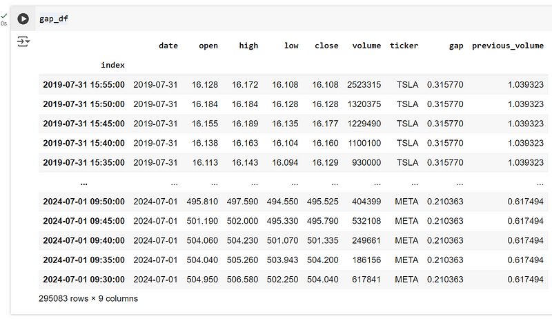
return df让我们拿一些热门股票(特斯拉、英伟达和 Meta 股票)来做例子:
使用这些函数后,我们就得到了这个数据帧(包含前一天价格差距和相对日成交量的数据):
三、计算基本指标
让我们用 Python 计算一些常用于定量分析的最重要的技术指标。在本示例中,我们将计算开盘突破策略的指标,该策略是最著名、最赚钱的日内交易技巧之一。该策略包括在开盘区间的涨跌幅限制时买入股票,可用于 2、5、15、30 或 60 分钟的区间。
可以使用以下代码计算移动平均线和成交量加权移动平均线,以及开盘区间的指标,如成交量、宽度、波动率等,这些指标对于了解开盘后第一分钟内股票的走势非常重要。
# Prepare the DataFrame with necessary calculations
def calculate_moving_averages(df):
    df['MA_5'] = df['close'].rolling(window=5).mean()
    df['MA_10'] = df['close'].rolling(window=10).mean()
    df['MA_20'] = df['close'].rolling(window=20).mean()

    # Adding the distance from moving averages as percentages
    df['distance_MA_5_pct'] = (df['close'] - df['MA_5']) / df['MA_5'] * 100
    df['distance_MA_10_pct'] = (df['close'] - df['MA_10']) / df['MA_10'] * 100
    df['distance_MA_20_pct'] = (df['close'] - df['MA_20']) / df['MA_20'] * 100

    return df

def calculate_vwap(df):
    df['VWAP'] = (df['volume'] * (df['high'] + df['low'] + df['close']) / 3).cumsum() / df['volume'].cumsum()
    return df

def prepare_dataframe(df):
    df.index = pd.to_datetime(df.index)
    df = calculate_moving_averages(df)
    df = calculate_vwap(df)
    return df

# Function to calculate indicators for each stock
def prepare_indicators(ticker, df, opening_range_duration):
    opening_range_df_list = []
    for day in df.index.normalize().unique():
        day_data = df[df.index.normalize() == day]

        # Ensure data is sorted by timestamp
        day_data = day_data.sort_index()

        if len(day_data) < opening_range_duration:
            continue

        # Select the correct opening range
        opening_range = day_data.iloc[:opening_range_duration]
        opening_range_high = opening_range['high'].max()
        opening_range_low = opening_range['low'].min()
        opening_range_close = opening_range['close'].iloc[-1]
        opening_price = opening_range['open'].iloc[0]
        opening_range_width = ((opening_range_high - opening_range_low) / opening_price) * 100
        opening_range_volatility = opening_range['close'].std() if opening_range_duration > 1 else 0
        opening_range_volume = opening_range['volume'].sum()
        opening_range_avg_volume = opening_range_volume / opening_range_duration

        post_opening_range = day_data.iloc[opening_range_duration:]

        breakout_idx = None
        breakout_type = None
        for idx in post_opening_range.index:
            if post_opening_range.loc[idx]['low'] > opening_range_high:
                breakout_idx = idx
                breakout_type = 'bullish'
                break
            elif post_opening_range.loc[idx]['high'] < opening_range_low:
                breakout_idx = idx
                breakout_type = 'bearish'
                break

        if breakout_idx is None:
            continue

        breakout_data = day_data.loc[breakout_idx]

        next_1_hour = day_data.loc[breakout_idx:].iloc[1:13]
        if breakout_type == 'bullish':
            max_price_next_1_hour = next_1_hour['high'].max() if not next_1_hour.empty else np.nan
            target = (max_price_next_1_hour - breakout_data['close']) / breakout_data['close'] * 100 if not np.isnan(max_price_next_1_hour) else np.nan
        else:
            min_price_next_1_hour = next_1_hour['low'].min() if not next_1_hour.empty else np.nan
            target = (breakout_data['close'] - min_price_next_1_hour) / breakout_data['close'] * 100 if not np.isnan(min_price_next_1_hour) else np.nan

        # Calculate percentage change of breakout close price from opening range close price
        price_change_during_breakout = (breakout_data['close'] - opening_range_close) / opening_range_close * 100

        # Calculate direction consistency in the opening range
        if breakout_type == 'bullish':
            direction_consistency = (opening_range['close'] > opening_range['open']).sum() / len(opening_range)
        else:
            direction_consistency = (opening_range['close'] < opening_range['open']).sum() / len(opening_range)

        # Calculate volume relative to the average volume during the opening range
        volume_relative_to_avg = (opening_range_volume - opening_range_avg_volume) / opening_range_avg_volume * 100

        # Calculate VWAP as a percentage relative to the close price
        vwap_end_pct = (breakout_data['VWAP'] - breakout_data['close']) / breakout_data['close'] * 100
        vwap_at_breakout_pct = (breakout_data['VWAP'] - breakout_data['close']) / breakout_data['close'] * 100

        row_data = {
            'ticker': ticker,
            'date': day,
            'opening_range_width': opening_range_width,
            'opening_range_volatility': opening_range_volatility,
            'direction_consistency': direction_consistency,
            'gap': df.loc[day_data.index[0], 'gap'],
            'previous_volume': df.loc[day_data.index[0], 'previous_volume'],
            'price_change_during_breakout': price_change_during_breakout,
            'volume_relative_to_avg': volume_relative_to_avg,
            'distance_MA_5_pct': breakout_data['distance_MA_5_pct'],
            'distance_MA_10_pct': breakout_data['distance_MA_10_pct'],
            'distance_MA_20_pct': breakout_data['distance_MA_20_pct'],
            'VWAP_End_pct': vwap_end_pct,
            'VWAP_at_Breakout_pct': vwap_at_breakout_pct,
            'breakout_type': breakout_type,
            'target': target
        }

        opening_range_df_list.append(row_data)

    return opening_range_df_list


# Apply the prepare_indicators function to each stock
def analyze_combined_data(df, opening_range_duration):
    opening_range_df_list = []
    for ticker in df['ticker'].unique():
        ticker_df = df[df['ticker'] == ticker]
        opening_range_df_list.extend(prepare_indicators(ticker, ticker_df, opening_range_duration))
    return pd.DataFrame(opening_range_df_list)
让我们看看它如何使用 15 分钟开仓区间策略的数据(即 5 分钟数据的 3 个区间):
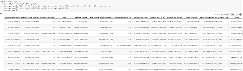
如您所见,我们在上面构建了一个非常全面的数据框架,使用了移动平均线等常用指标,以及其他对我们有意义的指标。在研究中,你只需问问自己,你想测试的假设是什么?在这种情况下,我们要测试的信念就是 ORB 策略中所包含的信念。
请注意,为达到目的,我创建了一个目标,用来衡量我们用这行代码买入看涨突破或卖出看跌突破后,在接下来的 60 分钟内可以获得的最大利润:
target = (breakout_data['close'] - min_price_next_1_hour) / breakout_data['close'] * 100 if not np.isnan(min_price_next_1_hour) else np.nan您可以根据自己的喜好进行调整,但通常 ORB 包括在突破后短时间内持仓。如果交易成功(股票向您期望的方向移动),就必须决定何时离场。
相反,如果交易与您的预期背道而驰,您就必须决定何时出局,在损失过大之前减少损失。
一般来说,日间交易者会选择 1:3 的风险与回报比例,这可能表示他们会在亏损 1%的时候平掉仓位,在盈利达到 3%的时候获利了结,或者他们会在亏损超过 0.5%的时候就平仓,在盈利超过 1.5%的时候赚一笔。
就是为何我们要研究你所能获取的最大利润,因为这是决定何为合理离场价格、对利润感到满足以及何种程度的亏损是我们能够接受或无法接受的关键要素。
通过数据研究,我们可以确定什么是真正的最佳值,并根据回溯测试做出明智的决定。
四、观点总结
现在,您不必因为博主这么说,就坚信开仓区间突破(或任何其他策略)是有效的。正确的量化思维应建立在对数据及自身研究充满信心的基石之上。那么,就让我们亲自来瞧瞧这个精美的数据框架所能告知我们的内容吧。
在理想的情况下,如果一只股票在开盘前大幅跳空上涨,成交量强劲,并且在上午继续朝同一方向上扬,没有丝毫犹豫(这就是我们测量波动率和方向一致性的原因),那么这只股票就很有可能在开盘后继续保持这种走势。现在,我们想知道数据是否支持这一理论,我们想知道这些股票按照我们假设的走势运行的概率。
我们需要探索变量和目标之间的关系,看看它们是否真的有影响,更重要的是,我们不仅要预测目标,还要衡量我们的预测结果有多好。
- 获取高质量数据是量化交易成功的关键。Alpha Vantage 提供了丰富的股票数据和已计算的指标,是量化分析的理想选择。
- 价格缺口和成交量是日内交易决策的重要指标。它们可以帮助交易者识别那些在开盘后可能出现大幅波动的股票。
- 开盘区间突破(ORB)策略是一种有效的日内交易策略。通过分析开盘区间的宽度、波动性、成交量和方向一致性等指标,可以更好地预测股票的走势。
- 风险与回报比率是交易决策的重要考量。日间交易者通常会选择 1:3 的风险与回报比率,并根据实际数据研究来决定何时进出市场。
延展阅读推荐
- 《手把手教你ai顾投:发现一个高质量的金融数据源》
- 《2024 年面向算法交易者的十大开源 Python 库》
- 《告别 backtrader!换这个库实施量化回测》
- 《借助算法交易,真的靠谱吗?》
- 《手把手教会你用 AI 和 Python 进行股票交易预测(完整代码干货)》
感谢您阅读到最后。如果对文中的内容有任何疑问,请给我留言,必复。
本文内容仅仅是技术探讨和学习,并不构成任何投资建议。
转发请注明原作者和出处。
Be First to Comment